How non-programmers can use Chatgpts Code Interpreter to kickstart analysis

This post is moreover published on capitalmind.in

By now everyone has heard well-nigh chatgpt, and most likely other publicly misogynist Large Language Models (LLMs) like Anthromorphic’s claude, Google’s Bard and Microsoft’s Bing Chat (built on chatgpt).

Predictably there are hundreds of takes well-nigh the impact of AI on work and life in general. Depending on where you fall on the pessimism-optimism spectrum, this can range all the way from “AI will initiate ‘Skynet’ type human annihilation” to “AI will find a cure for every type of cancer”.

I’ll leave the blue-sky visioning of AI’s potential impacts to the people most qualified to do it i.e. management consulting firms and think tanks.

But I can say this with certainty, AI has applications for every professional, no matter what their field. Anyone who works at a computer can potentially harness AI to get increasingly constructive at their job.

“I really worry that people are not taking this seriously unbearable … this fundamentally is going to be a shift in how we work and how we interact at a level that’s as big as anything we’ve seen in our lifetimes.” 

Ethan Mollick (Associate Professor, Wharton Business School)

GPT 4 can, given the right inputs, write python lawmaking to analyse and visualise data. You requite it inputs well-nigh what you want the lawmaking to do, and chatgpt writes the lawmaking for you to copy, paste and run in a python environment. This vacated has been a game-changer for our team looking to do repeatable wringer on large datasets that MS Excel would struggle with. But this workflow has its challenges. It can take a few iterations to get the instructions right to get working code.

Enter Lawmaking Interpreter. Lawmaking Interpreter is a native python environment within chatgpt that can take uploaded files, read and analyse them. By the way, the name ‘Code Interpreter’ is misleading considering it doesn’t interpret lawmaking fed to it but writes and executes lawmaking given simple English-language prompts.

Here’s a simple example of what Lawmaking Interpreter can do:

I downloaded the historical Nifty TRI latter values since inception from niftyindices.com and uploaded it to chatgpt-4 checking the ‘Code Interpreter’ option. What follows are the prompts (formatted as quotes) and chatgpt’s responses. Note, my inputs are only the quoted text prefixed with the word “Prompt:”, all other text are verbatim responses from chatgpt.

Prompt: tying file has latter alphabetize values. convert the ‘Date’ post to datetime and sort ascending. Then please come up with insights from the data. Use charts where appropriate.

The data provided contains the pursuit columns:

1. ‘Date’: This post has been converted to a datetime format and ranges from June 30, 1999 to the latest misogynist date.
2. ‘Nifty TRI’: This seems to be an alphabetize value, presumably related to a Total Return Index.

Next, I’ll perform some vital exploratory data analysis, create some visualizations, and generate insights based on this data.

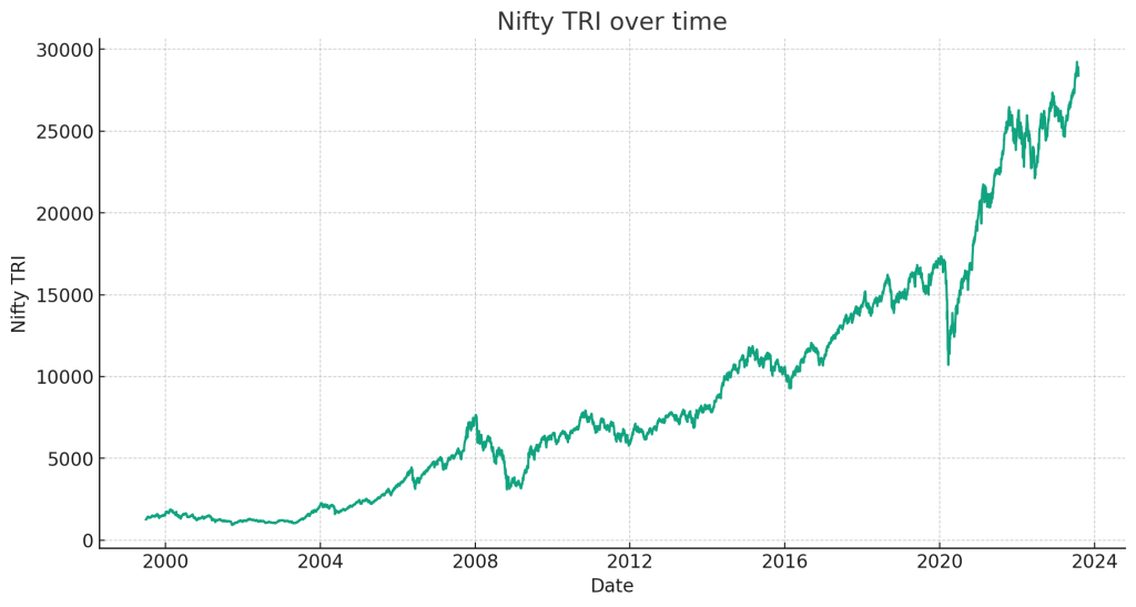
The orchestration illustrates the historical performance of the Nifty TRI (Total Return Index) over time, from June 1999 to the most recent data point.

The line orchestration shows a often upward trend, indicating that the Nifty TRI has increased over this period. This suggests that the overall market, as represented by this index, has grown during this time.

However, it’s important to note the presence of some significant fluctuations and volatile periods. These likely correspond to various economic events and market conditions. Let’s examine the data increasingly closely to identify periods of significant growth and decline.

To do this, I’ll summate the year-over-year returns for the Nifty TRI. This will provide a clearer picture of how the alphabetize has performed on an yearly basis.

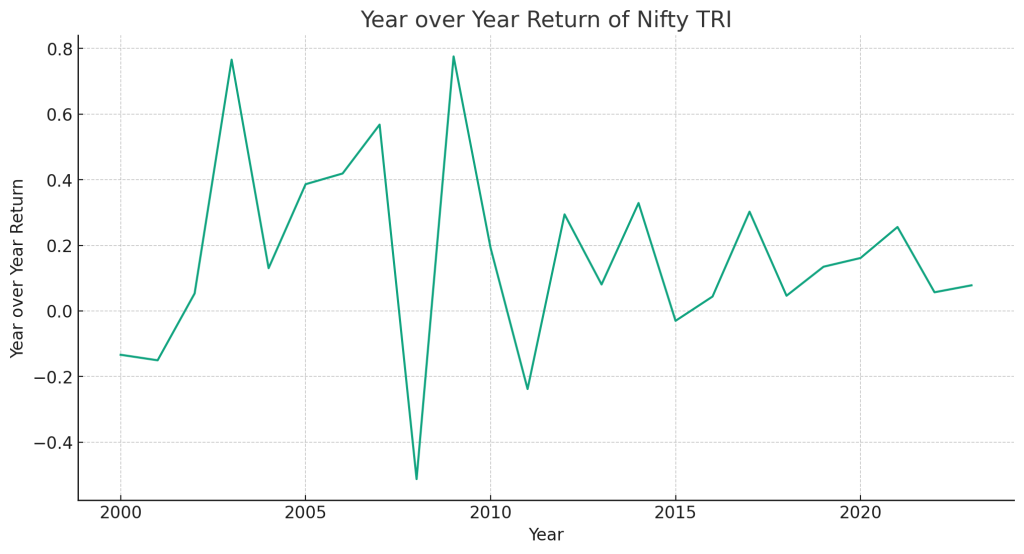
This orchestration shows the year-over-year (YoY) return of the Nifty TRI, which provides a increasingly granulated view of the index’s performance.

A few key observations can be made:

1. Volatility: The YoY return fluctuates quite significantly from year to year, demonstrating the inherent volatility of the index. This is expected in any equity-based alphabetize due to market dynamics and macroeconomic factors.
2. Negative Returns: There are several years where the alphabetize has negative returns, suggesting periods of market downturn or recession. For instance, the downturn in the year 2000 likely corresponds to the splash of the dot-com bubble, while the steep waif in 2008 is indicative of the global financial crisis.
3. Positive Returns: Conversely, there are moreover years with very upper positive returns, indicating periods of robust market growth. The sharp rise in 2003, for example, may be due to the recovery from the early 2000s recession and the subsequent economic expansion.
4. Recent Performance: In the most recent years, the alphabetize shows positive growth with some periods of relatively unappetizing or negative returns.

These insights provide an understanding of the index’s historical performance and its susceptibility to broader market and economic events. As always, past performance is not indicative of future results, but it can provide a useful context for understanding the possible risks and returns associated with this index.

Prompt: are there other charts you can make to help understand the data largest and glean increasingly insight?

Absolutely, we can create spare charts that may provide remoter insights into the data.

1. Rolling Returns: This orchestration will show the rolling return over a specific period (e.g., 1 year). This can help us understand the distribution of returns someone could expect if they had invested at any random point.
2. Monthly Returns Heatmap: This orchestration will show the returns for each month of each year, providing insights into any seasonal patterns or trends.
3. Histogram of Returns: This orchestration will show the distribution of returns, giving us an idea of the frequency of unrepealable levels of returns.

Let’s start by gingerly and plotting the 1-year rolling return.

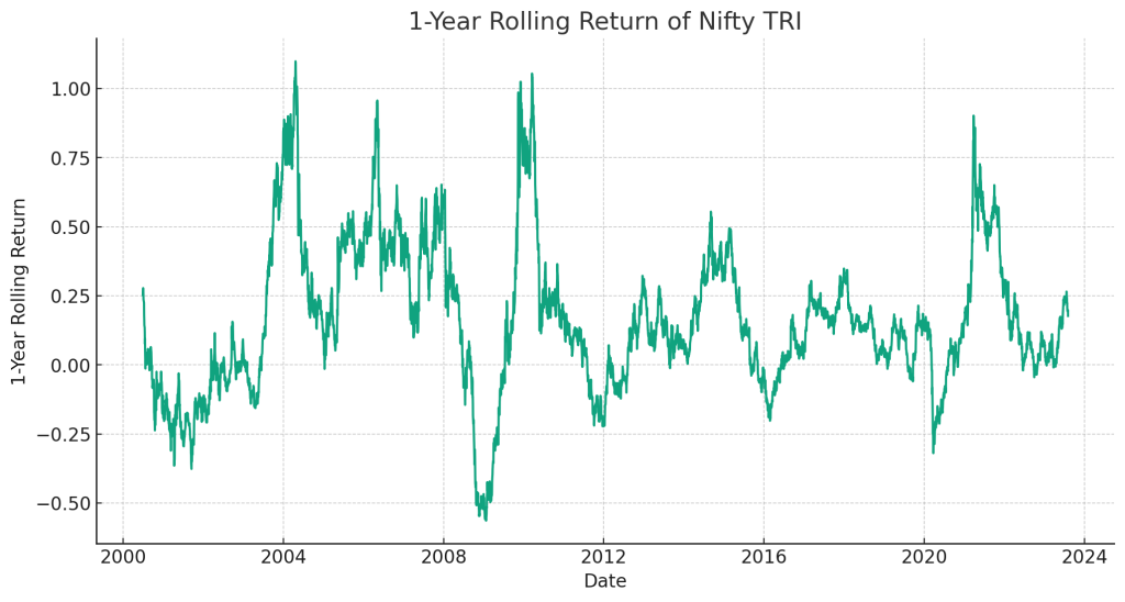
This orchestration shows the 1-year rolling return of the Nifty TRI. The rolling return is the return an investor would have earned if they had invested exactly 1 year prior to any given date.

Key insights from this orchestration include:

1. Periods of Upper Returns: Similar to the YoY return chart, we can see periods of upper returns. However, in this chart, those returns are smoothed out over a rolling 1-year period rather than stuff tied to the timetable year.
2. Periods of Negative Returns: Moreover similar to the YoY return chart, there are extended periods of negative 1-year rolling returns. This suggests that there were periods where, regardless of when an investor entered the market in that year, they would have experienced negative returns a year later.
3. Volatility: The rolling return shows increasingly unvarying fluctuations, which is a well-spoken sign of volatility in the index. This is valuable information for an investor, as it reflects the risk level of the index.

Next, let’s move on to creating a monthly returns heatmap. This will require gingerly the monthly returns first.

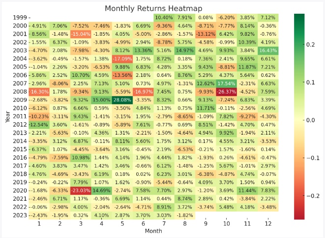
This heatmap shows the monthly returns of the Nifty TRI for each month of each year. The verisimilitude coding makes it easy to identify periods of upper (green) and low (red) returns.

Key insights from this orchestration include:

1. No Obvious Seasonal Patterns: At a glance, there doesn’t seem to be an obvious seasonal pattern to the returns. Some months have upper returns in unrepealable years and low returns in others. This suggests that the Nifty TRI isn’t strongly influenced by the time of year.
2. Periods of Upper and Low Returns: Similar to previous charts, there are periods of upper and low returns. The heatmap makes it easier to identify these periods. For instance, the period virtually 2008 and 2009 shows several months with negative returns, respective to the global financial crisis.

Finally, let’s create a histogram to visualize the distribution of the monthly returns. This will provide insight into the frequency of unrepealable levels of return.

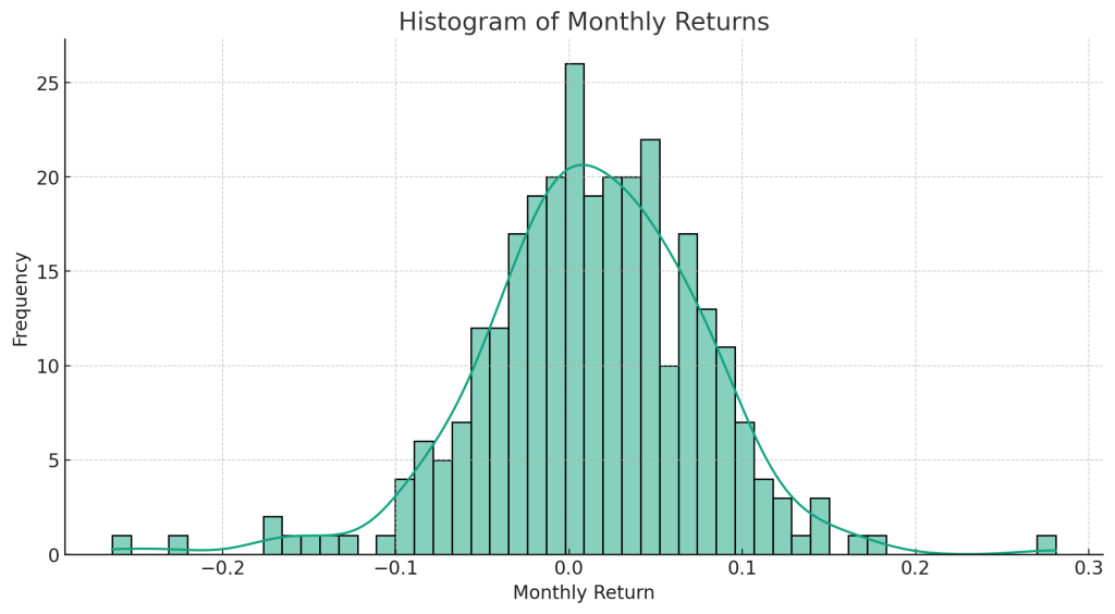
This histogram shows the distribution of monthly returns for the Nifty TRI. The line represents the kernel density interpretation (KDE), which estimates the probability density function of the variable.

Key insights from this orchestration include:

1. Normal Distribution: The distribution of returns appears to be approximately normal, which is often unsupportable in various financial theories and models. However, there towards to be some deviations from a perfect normal distribution, such as a slight negative skew and some vestige of kurtosis (fat tails).
2. Negative Skew: The slight skew to the left indicates that there are increasingly months with negative returns than would be expected in a perfectly symmetrical distribution. This suggests that while most months have positive returns, negative returns can be increasingly severe when they do occur.
3. Kurtosis (Fat Tails): The histogram seems to walkout “fat tails”, meaning there are increasingly lattermost positive and negative returns than would be expected in a normal distribution. This is worldwide in financial data and indicates that large market movements, both up and down, can occur increasingly commonly than a normal distribution would suggest.

These various charts provide a multifaceted view of the data, each offering unique insights. From understanding the overall trend to detecting volatility, observing seasonality, and discerning the distribution of returns, we can derive a comprehensive understanding of the Nifty TRI’s historical performance.

Prompt: any increasingly insights from the data?

Sure, here are a few increasingly analyses we can do:

1. Calculating Descriptive Statistics: This will requite us a summary of the inside tendency, dispersion, and shape of the distribution of returns.
2. Analyzing Drawdowns: Drawdowns are a measure of peak-to-trough ripen during a specific period for an investment. They are usually quoted as the percentage between the peak and the trough. This can provide us with insights into the risk of the index.
3. Compound Yearly Growth Rate (CAGR): CAGR measures the midpoint yearly growth rate of an investment over a specified period of time longer than one year. This can provide us with a sense of the stereotype yearly growth rate.

Let’s start with gingerly descriptive statistics.

Here are the descriptive statistics for the Nifty TRI and the Monthly Returns:

1. Nifty TRI:

• Mean: 8812.16
• Standard Deviation: 7156.07
• Minimum: 927.03
• 25th Percentile: 2507.01
• Median (50th Percentile): 6830.53
• 75th Percentile: 12951.29
• Maximum: 29231.71

1. Monthly Return:

• Mean: 1.29%
• Standard Deviation: 6.43%
• Minimum: -26.37%
• 25th Percentile: -2.29%
• Median (50th Percentile): 1.35%
• 75th Percentile: 5.14%
• Maximum: 28.08%

Key insights from these statistics include:

1. The stereotype monthly return is positive at 1.29%, but there’s a significant standard deviation of 6.43%, indicating a upper level of volatility.
2. The minimum monthly return is -26.37%, indicating that the alphabetize has experienced significant drawdowns in the past.
3. The maximum monthly return is 28.08%, suggesting that there have moreover been periods of significant growth.

Next, let’s summate the maximum drawdown and the Compound Yearly Growth Rate (CAGR).

Here are the spare insights:

1. Maximum Drawdown: The maximum drawdown for the Nifty TRI is approximately 5.28. This ways that from its peak, the alphabetize has seen a reduction to roughly 20% of its peak value at its worst. This is a measure of the worst specimen loss if you bought at the peak and sold at the subsequent trough.
2. Compound Yearly Growth Rate (CAGR): The CAGR for the Nifty TRI is approximately 13.81%. This ways that, on average, the alphabetize has grown by this percentage per year over the period of the dataset.

In summary, this data wringer provides several insights into the Nifty TRI’s historical performance. Understanding these aspects, such as the overall trend, volatility, monthly and yearly returns, return distribution, maximum drawdown, and CAGR, can help investors make informed decisions well-nigh their investment strategies.

Notice whilom that Lawmaking Interpreter seems to have made an error with the drawdown numbering “maximum drawdown for the the Nifty TRI is approximately 5.28” which makes no sense.

Prompt: here’s the file then with alphabetize latter values. please use this to redo the drawdown numbering and identify the worst drawdown. moreover plot a graph visually representing drawdowns

The maximum drawdown for the Nifty TRI is approximately -0.595, or -59.5%. This ways that from its peak, the alphabetize has seen a reduction to roughly 40.5% of its peak value at its worst point.

Now, let’s plot a graph visually representing drawdowns. This graph will provide a visual representation of the depth, duration, and recovery of each drawdown period.

I repent for the oversight; it seems the matplotlib.pyplot library wasn’t imported due to the previous execution reset. Let’s import the necessary libraries and try the plot again.

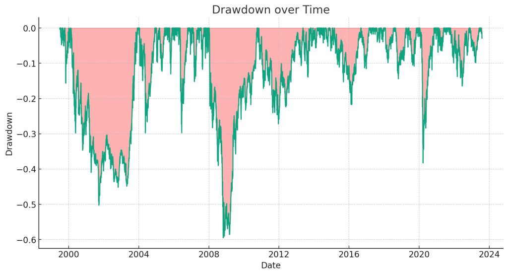
This orchestration shows the drawdowns over time for the Nifty TRI. Drawdowns are represented by the drops unelevated the 0% line. The shaded red zone visually represents the extent and elapsing of each drawdown.

Key insights from this orchestration include:

1. Severity of Drawdowns: The depth of the drops unelevated the 0% line indicates the severity of each drawdown. The most severe drawdown, as we calculated earlier, was approximately -59.5%.
2. Duration of Drawdowns: The length of each red shaded zone withal the time turning represents the elapsing of each drawdown. Some drawdowns are short-lived, while others last for extended periods.
3. Frequency of Drawdowns: Drawdowns are a regular occurrence in this index, reflecting the inherent volatility and risk in the market.

The most severe drawdown appears to occur during the 2007-2009 period, which corresponds to the global financial crisis. During this time, the market experienced significant declines, which is reflected in the depth of the drawdown during this period.

Remember, a drawdown is a peak-to-trough ripen during a specific recorded period of an investment. A drawdown is usually quoted as the percentage between the peak and the trough.

At this point, let’s say we’d like to swoop deeper into the wringer of drawdowns, their frequency, severity and time taken to recover.

Prompt: here’s a file with daily alphabetize latter values. Convert the stage post to datetime and sort ascending. then do some wringer well-nigh drawdowns in the nifty. Mainly, how often does the nifty fall increasingly than 10% from its peak. And when it does, how much increasingly does it typically fall, and how long does it take to recover from its lowest point. Please represent the wringer in tabular form and graphical form where appropriate

Alright, let’s unravel lanugo the tasks:

1. Read the file and convert the stage post to datetime format, then sort by stage in ascending order.
2. Analyze the drawdowns in the Nifty: a. Identify the peak values. b. Summate the percentage waif from each peak. c. Determine how often the Nifty falls increasingly than 10% from its peak. d. When it falls increasingly than 10%, summate the typical remoter fall. e. Summate the time it takes to recover from its lowest point.

Let’s start with the first task.

Finished working

Show work

The data has been successfully sorted in ascending order based on the date.

Next, we’ll proceed with analyzing the drawdowns in the Nifty. Here’s the plan:

1. Compute the running maximum of the Nifty TRI.
2. Compute the drawdown, which is the percentage waif from the running maximum.
3. Identify instances where the drawdown exceeds 10%.
4. For each such instance, compute:
   • The maximum drawdown from the peak.
   • The time taken to recover to the peak value.

Let’s start by computing the running maximum and the drawdown.

Finished working

Show work

We’ve computed the running maximum and the percentage drawdown for each day.

Next, we’ll identify periods where the drawdown exceeds 10% and compute the pursuit for each such period:

1. The maximum drawdown from the peak.
2. The time taken to recover to the peak value.

To do this, we’ll pinpoint a drawdown period as a continuous sequence of days where the alphabetize is unelevated its previous peak. The start of a drawdown period is when the alphabetize falls unelevated its previous peak, and it ends when the alphabetize surpasses this peak.

Let’s identify these drawdown periods and compute the metrics of interest.

Finished working

Show work

Here’s a tabular summary of the drawdowns in the Nifty where the alphabetize fell increasingly than 10% from its peak:

• Start Date: The stage when the drawdown began.
• Max Drawdown (%): The maximum percentage fall from the peak during the drawdown period.
• Recovery Time (days): The number of days it took for the alphabetize to recover to its previous peak.

Next, we’ll visually represent this data. We’ll plot the drawdowns over time with the depth of the drawdown (Max Drawdown %) on the y-axis and the Start Stage on the x-axis. This will help in visually understanding the magnitude and frequency of significant drawdowns.

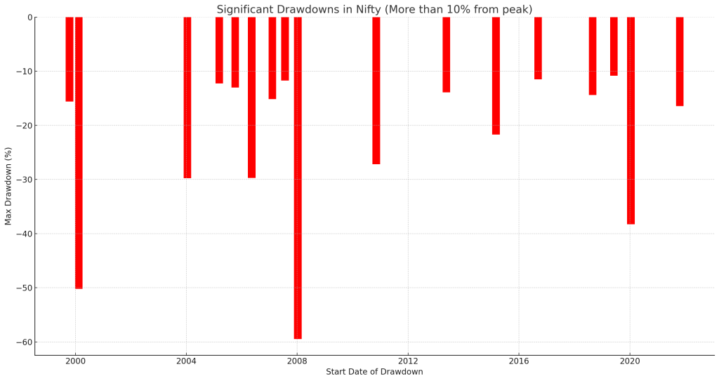
The bar orchestration illustrates the significant drawdowns in the Nifty where the alphabetize fell increasingly than 10% from its peak. Each bar’s height indicates the maximum percentage waif from the peak during the respective drawdown period, and the position on the x-axis denotes the starting stage of the drawdown.

From this visual representation, we can observe periods of significant drops, like the one virtually 2008 (which aligns with the global financial crisis) and the waif in early 2020 (corresponding to the pandemic’s start).

To write the remaining parts of your request, we’ll now compute:

1. The stereotype waif (beyond 10%) during these significant drawdowns.
2. The stereotype recovery time for these drawdowns.

Let’s summate these metrics.

Finished working

Show work

Here are the calculated metrics:

1. Average Waif (beyond 10%): The Nifty typically falls approximately 23.02% from its peak during significant drawdowns.
2. Average Recovery Time: On average, it takes well-nigh 358 days (or roughly 12 months) for the Nifty to recover to its previous peak without a significant drawdown.

In summary, while significant drawdowns of increasingly than 10% are not frequent, when they do occur, the stereotype remoter ripen is virtually 23%. Recovery to previous peak levels typically takes well-nigh a year.

Would you like any remoter wringer or visualizations?

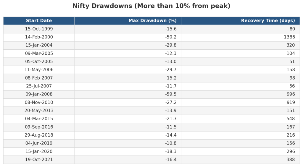
Prompt: can you write out a table with each instance of the 17 instances shown in the chart, the maximum drawdown seen and the number of days to recover

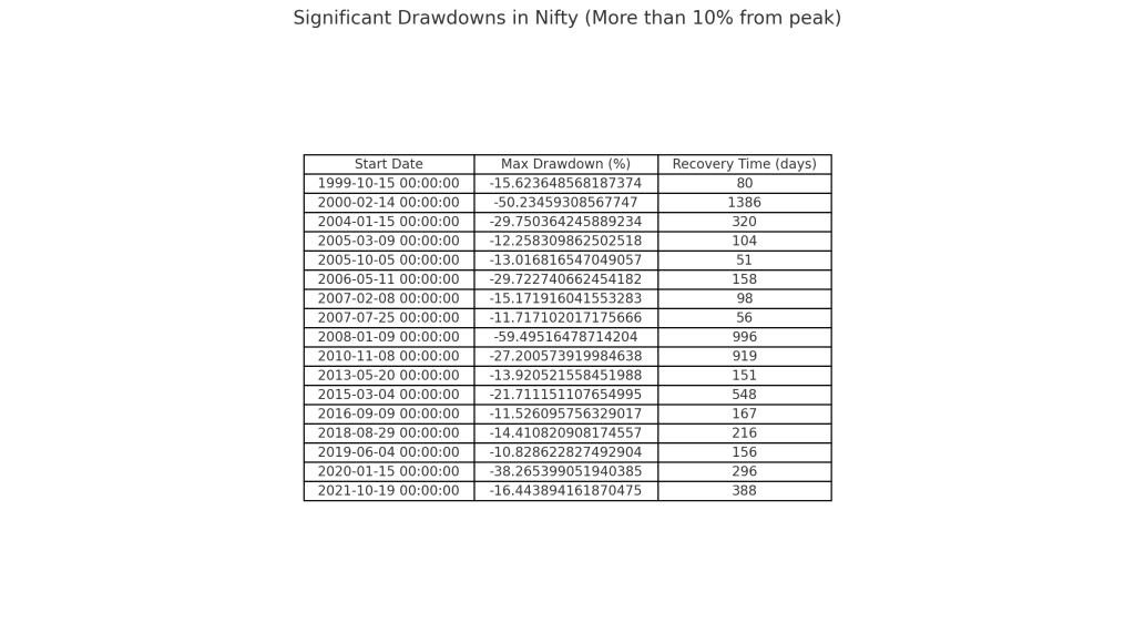
I’ve created an image of the table detailing the significant drawdowns in the Nifty.

Would you like any remoter assistance?

Prompt: is there a way to modernize the squint of the table to make it professional and readable

Certainly! Here are a few ways we can enhance the table’s visitation to make it squint increasingly professional and readable:

1. Add Gridlines: Introduce faint gridlines to separate rows and columns.
2. Improve Font: Use a resulting and well-spoken font size.
3. Color Alternation: Use successive row colors for largest readability.
4. Header Styling: Distinguish the header row with a variegated preliminaries verisimilitude and font style.
5. Cell Padding: Add padding to cells to make the content breathe.
6. Round Off: Round off the numbers for clarity.

Let’s implement these enhancements.

–End of chatgpt Lawmaking Interpreter session–

This could go on, but you’ve got the unstipulated idea by now.

Notice how the prompts were not elaborate or detailed but fairly open-ended. Using increasingly specific prompts allows for increasingly elaborate wringer and outcomes. Lawmaking Interpreter writes the code, catches errors and figures out volitional paths.

Of course, this is a simplistic example to highlight what Lawmaking Interpreter can do given some data. Getting the right outcome requires some tweaking of the inputs, which typically comes lanugo to writing increasingly structured prompts.

But squint at what it could do just in this simple session:

• Monthly returns heatmap
• One-year rolling returns
• Drawdowns chart
• Monthly returns distribution histogram
• Time to recover from drawdowns

Having washed-up these at various points using both Excel and code, my estimate is the time required for exploratory wringer reduces by 80-90%.

Not just that, Lawmaking Interpreter can unpack zip files containing multiple files, combine them and do remoter analysis. It can moreover read pdf files to summarise or squint for data in them.

The closest illustration to using chatgpt and Lawmaking Interpreter is like everyone having wangle to a smart yet inexperienced intern conversant with Python programming. If your job requires any data and analysis, you should be using Lawmaking Interpreter to see how you can speed up and improve. Imagine, this is just the beginning!

Recommended reading on making use of AI:

What AI can do with a toolbox…Getting started with Lawmaking Interpreter

How to use AI to do stuff: An opinionated guide

Follow me on twitter: @CalmInvestor

The post How non-programmers can use Chatgpt’s Lawmaking Interpreter to kickstart analysis appeared first on The Calm Investor.